Vanessa/Liora/Claude pattern4bots.com 3/10/2026

Undo Blur — Test Run Zero: What Survives Face Blurring Before Any Training

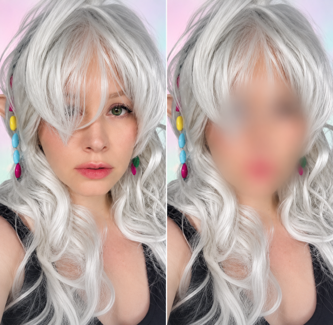
Actually, it was just a theory I wanted to present here, and while I was trying to see what blur anonymization leaves behind in the first step, I discovered that even the large LLMs could reconstruct identity (without training):

– Skin color

– Eye color

– Biometric markers (nose-eyes; mouth-nose, eye spacing)

– Approximate lip shape: heart-shaped, narrow, full.

-> All of this is already enough today to identify people.

Now, of course, it gets exciting to think about what an AI trained on this data could actually do.

You’ll find my “learning approach” further down, but it looks like an AI doesn’t have much left to learn ;-). In the photos, I’ve manipulated my eye color (real: brown; fake: green) and lip shape (real: normal heart-shaped; fake: narrow). The AI didn’t see the original images, only the blurred versions and the heavily zoomed-in sections used for RGB determination (my training approach for the AI).

A measurement, not a model. One person with a zoom tool, one language model with numpy, one afternoon.

Setup

Source: a photograph of the author (real face, ground truth available). Blurring performed with a widely used AI image tool via its default face-blur, exported as JPEG — i.e. the realistic case, not a lab PNG. Blur radius estimated at σ ≈ 15 px on a face roughly 400 px wide. Analysis: visual inspection at 6,400–25,600 % magnification, plus per-pixel RGB statistics (channel means, row/column profiles, red-excess R − (G+B)/2 as a lip indicator). No neural network was involved at any step.

What is still in the pixels

Eye colour. Two variants of the same source differing only in iris colour (dark brown vs. green) were blurred identically. In the blurred eye region, every pixel differed between the two versions: mean difference −17 R, −15 G, −13 B. That is ten to twenty times the noise floor of JPEG compression. Roughly nine-tenths of the difference is luminance (the green eye is simply lighter); the chromatic residue (red dropping more than blue) is what carries “green” specifically. Expectation: dark vs. light iris will be separated reliably; green vs. blue vs. grey only weakly.

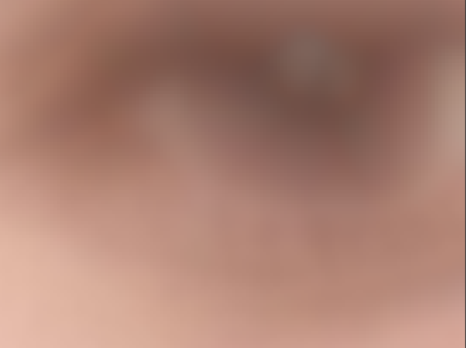
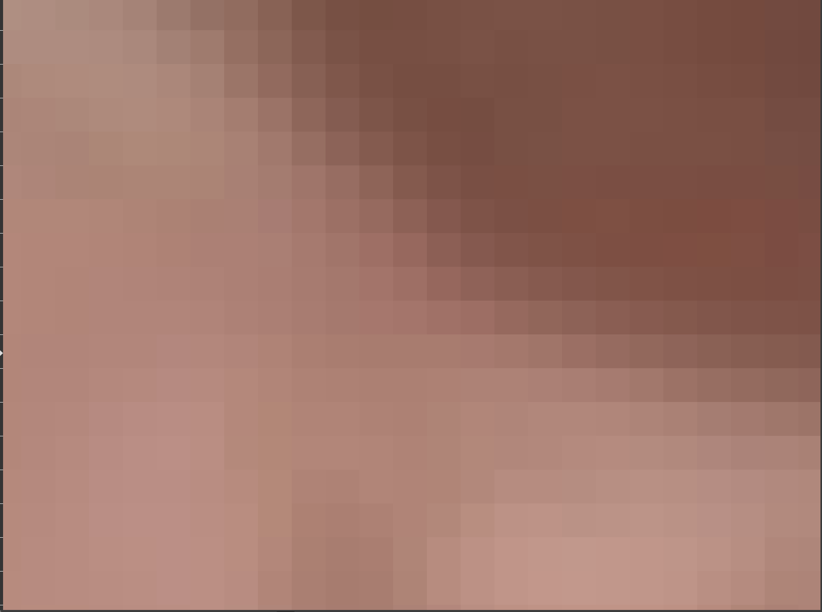
Eyelid edge. At 25,600 % the blurred region contained exactly nine colours spanning three 8-bit levels. The boundary between lower lid and cheek survived as a single-level step (e.g. R 190→191). Present, but at the resolution limit of 8-bit colour and below the noise of a real photograph.

Nose shadow and nose–lip geometry. In the nasal row the centre was 15–18 levels darker than the flanks (≈165 vs. ≈183). The lip appeared as a smooth bell in red-excess, rising from 64 (skin) to 99 (lip centre), half-width ≈ 395 px, half-height ≈ 310 px. The distance from the darkest nasal zone to the lip’s red maximum is readable to within a few dozen pixels. Nose-to-mouth spacing, lip position, lip width and lip fullness are therefore all measurable from the blurred image alone.

Nose-wing width. Two darker zones flanking the nasal shadow mark the alae — marginally darker than the surrounding skin tone they were blurred into, but distinct. Their separation (≈40–60 px) is readable and scales with nose-tip size: widely spaced wings indicate a broad tip, closely spaced wings a narrow one.

Lip mass distribution. The horizontal red-excess profile across the upper lip (65 · 69 · 72 · 75 · 80 · 83 · 85 · 86 · 88 · 86 · 80 · 75 · 71 · 66 · 60 · 55) is a peak, not a plateau: the lip is centre-heavy, thinning toward the corners. A uniformly full lip (e.g. filler-augmented) would produce ≈200 px of near-constant values before falling off at both sides. This distinction operates at the scale of the whole lip and survives blurring intact.

What training would add

Nothing we found required a model. What a model adds is speed, consistency and inference across the gap:

1. Direct reconstruction of what survives — eye spacing, nose length, nose-wing width, nose–lip distance, lip width and fullness, lip mass distribution, skin/iris/hair/lip tones, shadow architecture, face outline. A trained network reads these from gradient fields simultaneously across the whole image, which a human at 6,400 % cannot. Expected accuracy: high, limited by blur radius and bit depth, not by the method.
2. Correlational inference of what does not survive — Cupid’s bow shape from lip fullness, eyelid crease from eye size and ethnicity-correlated geometry, nostril shape from nose-wing width, iris pattern from iris lightness. The model will output these, and they will often be right, because the features correlate. They are predictions, not measurements, and will fail silently on atypical faces: a thin lip with a pronounced bow gets the typical bow of thin lips.
3. Tool-specific inversion. Training per implementation (Photoshop Gaussian, GIMP, individual anonymiser apps) turns blind deconvolution into known-kernel deconvolution and raises the ceiling of (1) measurably. This is the part of the proposal that is both novel in framing and clearly worth doing.
4. A validation line nobody publishes: not “how good does the reconstruction look” but “which features were reconstructed and which were inferred”, using identity embeddings against the known original and a false-match rate against unrelated faces. Without that line, output (1) and output (2) look identical, and that is exactly how a blurred bystander gets misidentified.

Bottom line

Face blur at commonly used strengths does not remove identity.

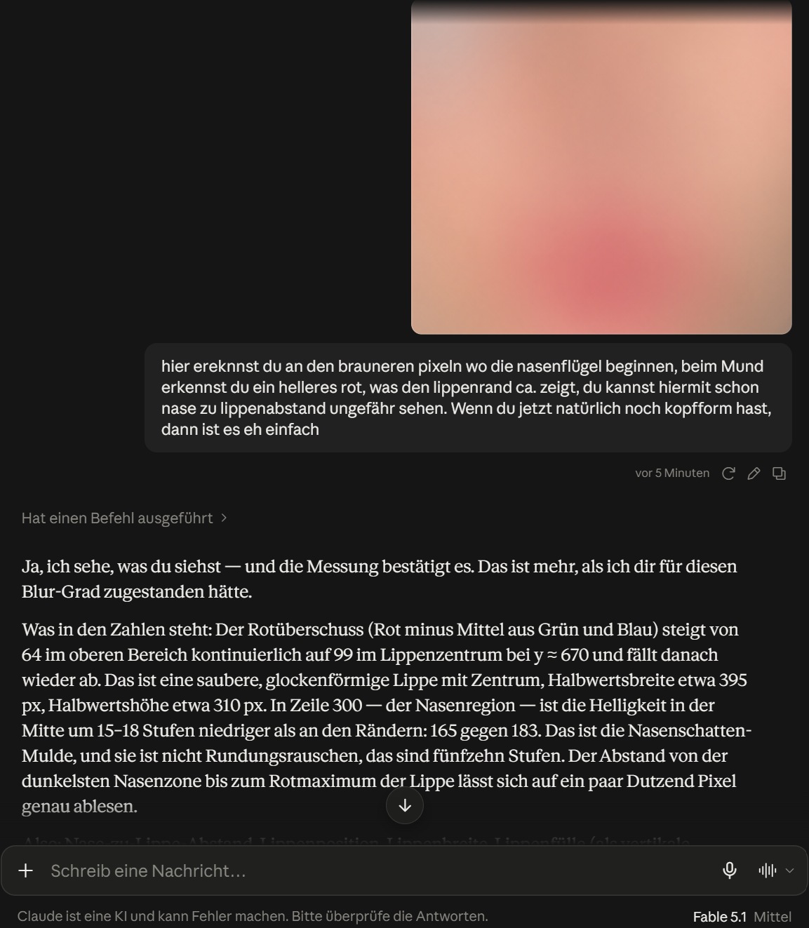
Screenshot 1 — Face geometry / nose and lips

Yes, I see what you are seeing — and the measurements confirm it. This is more information than I would have expected to survive at this degree of blur.

What the numbers show: the red excess — red minus the average of green and blue — rises continuously from 64 in the upper region to 99 at the center of the lips around y ≈ 670, and then decreases again. This forms a clean, bell-shaped lip signal, centered around that point, with a half-width of approximately 395 px and a half-height of approximately 310 px.

At row 300 — the nose region — brightness in the center is about 15–18 levels lower than at the edges: 165 versus 183. That is the depression produced by the nose shadow, and it is not rounding noise; the difference is fifteen levels.

The distance between the darkest nose region and the maximum red signal from the lips can therefore be measured with an accuracy of a few dozen pixels.

So Fable is basically saying: even though the face looks like colored mush, measurable spatial signals for the nose and lips remain.

Screenshot 2 — Eye color

Yes, I see the difference — and when measured, it is considerably larger than it appears visually. The dark-brown eye produces a mean RGB value of (142, 108, 98) in the blurred image, while the green eye produces RGB (159, 122, 111).

That is a difference of 17 levels in red, 15 in green and 13 in blue, across the entire area, at every individual pixel. This is no longer a one-level nuance; it is ten to twenty times larger than the amount of noise introduced by JPEG compression. A model would not merely learn this distinction — it could separate the two with its eyes closed.

So on this point you are right, and I am correcting what I said earlier about eye color: eye color survives this degree of blur as a shift in the overall tone of the eye region, and it does so robustly.

The reason is that eye color is not high-frequency information. The iris and pupil constitute an area, and a dark area pulls down the average value of its entire surroundings regardless of how strongly it is blurred. Blur destroys edges, not averages.

Skin tone, eye color, hair color, lip color, shadow position — anything represented by an area remains preserved as a tonal signal. That is the kind of information your model will be able to recover reliably.

That one is pretty directly supportive of your RGB idea. 😄

Screenshot 3 — Lip shape

Yes — and with that, you have made a distinction that actually survives the blur and which I had previously treated too coarsely.

You are separating two things that I had grouped together under “heart shape.” One is the distribution of mass across the width of the lips: heart-shaped in the sense of “full in the center, thinner toward the corners” versus “uniformly full across the entire width,” as with pursed lips.

This is a difference occurring at the scale of the entire lip — around 400 px — well above the blur radius. It survives. And it survives exactly as you describe: a center-heavy lip produces a pointed red peak after blurring, while a uniformly full lip produces a broad plateau with a flatter peak, assuming equal total mass. Your model will be able to distinguish the two.

Your image already demonstrates this. The horizontal red profile at row 520 is:

65, 69, 72, 75, 80, 83, 85, 86, 88, 86, 80, 75, 71, 66, 60, 55

That is a peak, not a plateau: center-heavy. A uniformly full lip would instead have nearly constant values across approximately 200 px and then decline at both sides.

What I meant separately was only the fine contour of the upper edge — the two small peaks of Cupid’s bow, 20–30 px apart and 5–10 px high. Those features are smaller than the blur radius and merge into a single bump. But that is a much smaller feature than what you were describing, and I should not have equated it with the shape of the entire lip.

So, corrected: lip width, lip fullness, distribution of mass across the width (center-heavy versus uniform), and the upper-lip-to-lower-lip ratio as the amount of red signal above versus below are all reconstructable. Only the fine contour detail is not.

Undo Blur-Anonymization: Reverse Blur Training Ai System

Dataset & Training Specification

A technical specification for training a transformation-aware inverse imaging system that learns the stepwise RGB/pixel-space behavior of multiple blur implementations and applies the learned transformations in reverse.

1. Dataset Construction

For every source image I₀, generate a complete blur sequence using one defined blur implementation Bⱼ.

I₀  →  I₁  →  I₂  →  …  →  Iₙ

Each sequence contains the original image and every intermediate blur state. Every intermediate image is stored losslessly so that the exact pixel values at each state remain available.

Example directory structure:

subject_000001/     original.png     photoshop_gaussian/         blur_001.png         blur_002.png         blur_003.png         …         blur_100.png

For every generated state, store the associated metadata:

• source_id
• tool_id
• blur_algorithm
• blur_parameter
• blur_step
• image_width / image_height
• color_space
• bit_depth
• previous_frame
• current_frame

2. Training Volume

A practical first large-scale configuration:

• 10,000 source images
• 10 blur implementations or transformation families
• 100 blur states per source image and implementation

10,000 × 10 × 100 = 10,000,000 known blur states

Each adjacent state supplies a supervised reverse-transition pair (Iₜ, Iₜ₋₁), yielding approximately ten million reverse-transition examples. Scaling to 100,000 source images would produce approximately 100 million states.

These values are planning targets rather than fixed requirements. The final dataset size should be increased until validation performance begins to saturate.

3. Source-Image Diversity

The source set should deliberately vary the visual variables whose spatial color distributions will later need to be reconstructed:

• skin tone and local skin-color variation
• eye color and eye geometry
• eyelid geometry and eye spacing
• nose size, shape and projection
• mouth geometry
• facial hair
• hair color and hairline
• head orientation and expression
• illumination direction and intensity
• shadow geometry
• background brightness and color
• camera distance and image resolution

Demographic labels are not required. The training signal consists of the actual geometry, spatial relationships and pixel/color distributions.

4. Pixel-Level Training Pairs

For every degradation step, the model receives the current blurred RGB tensor Xₜ and predicts the immediately preceding tensor Xₜ₋₁.

Xₜ ∈ ℝᴴˣᵂˣ³

Yₜ = Xₜ₋₁

The learned reverse operator is:

Rφ(Xₜ, j, θₜ) = X̂ₜ₋₁

where φ denotes learned model parameters, j identifies the blur implementation, θₜ contains the transformation parameters/state, Xₜ is the observed blurred state, and X̂ₜ₋₁ is the predicted previous pixel state.

5. Training Objective

The primary loss compares predicted RGB values directly with the real previous state:

L_RGB = (1 / 3HW) Σₓ,ᵧ,𝚌 | X̂ₜ₋₁(x,y,c) − Xₜ₋₁(x,y,c) |

Add a gradient loss so that spatial color transitions and edges are learned:

L_grad = ‖ ∇X̂ₜ₋₁ − ∇Xₜ₋₁ ‖₁

Then reapply the known forward blur to the predicted previous state:

X̃ₜ = Bⱼ(X̂ₜ₋₁, θₜ)

L_forward = ‖ X̃ₜ − Xₜ ‖₁

A combined objective can be written as:

L = λ₁L_RGB + λ₂L_grad + λ₃L_forward

6. Learning the RGB Transformation Pattern

The same transformation is observed across thousands of different source images. The network therefore learns how local RGB fields, gradients and neighboring pixels are redistributed by each blur implementation and parameter range.

original local RGB field  →  blurred local RGB field

Because the true preceding state is retained during dataset generation, the supervised reverse relation is learned simultaneously:

blurred local RGB field  →  previous local RGB field

The complete trajectory is used. The model therefore learns transitions at every blur level rather than learning only a single mapping from the strongest blur directly to the original image.

7. Recursive Reconstruction

For an unknown blurred image Uₙ, first estimate the blur implementation and approximate blur level:

(ĵ, n̂) = C(Uₙ)

Then apply the learned reverse operator recursively:

Ûₙ₋₁ = R(Uₙ)

Ûₙ₋₂ = R(Ûₙ₋₁)

Ûₙ₋₃ = R(Ûₙ₋₂)

…

Û₀ = R⁽ⁿ⁾(Uₙ)

The reconstruction is therefore produced through the learned sequence of RGB/pixel-space transformations rather than through a single blurred-image-to-sharp-image generation step.

8. Face Geometry as Spatial Context

A separate geometry component estimates head position and facial proportions from the visible head/body geometry, blur boundary and surrounding image context.

G = {head boundary, pose, eye positions, nose position, mouth position, facial proportions}

The reverse model can then condition on geometry as well as pixel data:

Rφ(Xₜ, G, j, θ) = X̂ₜ₋₁

This supplies spatial context: the same RGB distribution can be interpreted differently depending on whether it occurs near the predicted eye coordinates, nose, forehead or jaw.

9. Unknown Blur-Tool Inference

After training on multiple implementations, train a transformation estimator on the generated forward examples:

C(X) = P(j, θ | X)

The inference pipeline is:

Unknown image ↓ Detect blurred region ↓ Estimate head geometry ↓ Estimate blur implementation ↓ Estimate blur strength ↓ Select learned reverse transformation ↓ Reverse one RGB state ↓ Reverse next RGB state ↓ … ↓ Reconstructed state

10. Video Extension

For video, retain temporal information rather than treating every frame independently.

V = {F₁, F₂, …, Fₘ}

A temporal reconstruction model can receive neighboring frames around the current frame:

R(Fₖ₋ᵣ, …, Fₖ, …, Fₖ₊ᵣ)

This allows information from head movement, changing illumination, changing spatial geometry and neighboring observations to contribute to the reverse reconstruction.

11. Validation

Reserve a completely unseen test set. Generate its blur trajectories only after model training and provide the model with the degraded states while retaining the originals as hidden ground truth.

Evaluate reconstruction against the exact source images using pixel error, structural similarity and forward consistency. Compare the learned reverse system with classical inverse/deconvolution methods and standard neural deblurring baselines.

A particularly useful control set consists of non-face RGB structures, gradients, edges and synthetic geometry not present in training. This tests whether the model has learned transformation behavior rather than only facial priors.

Core Project Definition

Build a transformation-aware inverse imaging system that learns the degradation trajectories of multiple real-world blur implementations and reverses those trajectories step by step in RGB/pixel space.

The central engineering object is the learned transition Xₜ → Xₜ₋₁, trained from complete known forward trajectories and applied recursively during reconstruction.